updated at 2021-02-26 by wojtek at bitologia.org (index)


plasma

Iterative (slow and unefficient) solution based on the diamond-square algorithm.

  1. allocate square lattice P of size L=2^N+1 for N = 2, 3, 4, ... ; here N = 3 and L = 8+1
  2. step S = 0: initialize corners
           P[0][0] = random value
           P[0][L] = random value
           P[L][0] = random value
           P[L][L] = random value
  3. in every next step S = 1, 2, 3, ...
    1. divide the appropriate area of P onto 4 smaller rectangles (here squares)
    2. apply the "d-s" algorithm to each sub-rectangle

      simply, in every step S one has 4^(S-1) sub-rectangles of size (L-1)/2^(S-1) each, sitting at positions [(L-1)*j/2^(S-1), (L-1)*k/2^(S-1)] for j and k = 0, 1, ... 2^(S-1)-1

      next, for each sub-rectangle:
      * ["d"] its center is a mean value of its four vertices
      * ["s"] the center of each side is a mean value of its three closest (euclidean) neighbours

      such order guarantees that the "s" part always has three elements to take the average, moreover, adding decreasing noise = noise(S) makes it more realistic

      example 4-step process for N = 3: points calculated at each step are numbered accordingly
             S=0                  S=1
             0 . . . . . . . 0    0 . . . 1 . . . 0
             . . . . . . . . .    . . . . . . . . .
             . . . . . . . . .    . . . . . . . . .
             . . . . . . . . .    . . . . . . . . .
         P = . . . . . . . . .    1 . . . 1 . . . 1
             . . . . . . . . .    . . . . . . . . .
             . . . . . . . . .    . . . . . . . . .
             . . . . . . . . .    . . . . . . . . .  
             0 . . . . . . . 0    0 . . . 1 . . . 0
      	
             S=2                  S=3
             0 . 2 . 1 . 2 . 0    0 3 2 3 1 3 2 3 0
             . . . . . . . . .    3 3 3 3 3 3 3 3 3
             2 . 2 . 2 . 2 . 2    2 3 2 3 2 3 2 3 2
             . . . . . . . . .    3 3 3 3 3 3 3 3 3
         P = 1 . 2 . 1 . 2 . 1    1 3 2 3 1 3 2 3 1
             . . . . . . . . .    3 3 3 3 3 3 3 3 3
             2 . 2 . 2 . 2 . 2    2 3 2 3 2 3 2 3 2
             . . . . . . . . .    3 3 3 3 3 3 3 3 3
             0 . 2 . 1 . 2 . 0    0 3 2 3 1 3 2 3 0
  4. repeat steps S until resolution limit is reached
  5. store data in file
  6. visualize

For non-square lattices one needs to implement fitting/rescaling procedure.

QBasic source is wickedly slow, although it is possible to watch the final effect:
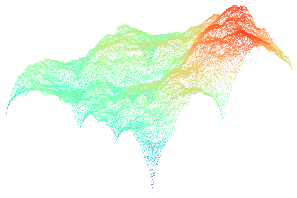
Fig. 1. Plasma in motion.

3-D variations

Generic picture for a 513 × 513 lattice generated by the C code and visualised with gnuplot

	$ gnuplot
	set palette rgb 33,13,10
	splot 'plasma02.dat' with points palette pt 4 ps 0.5

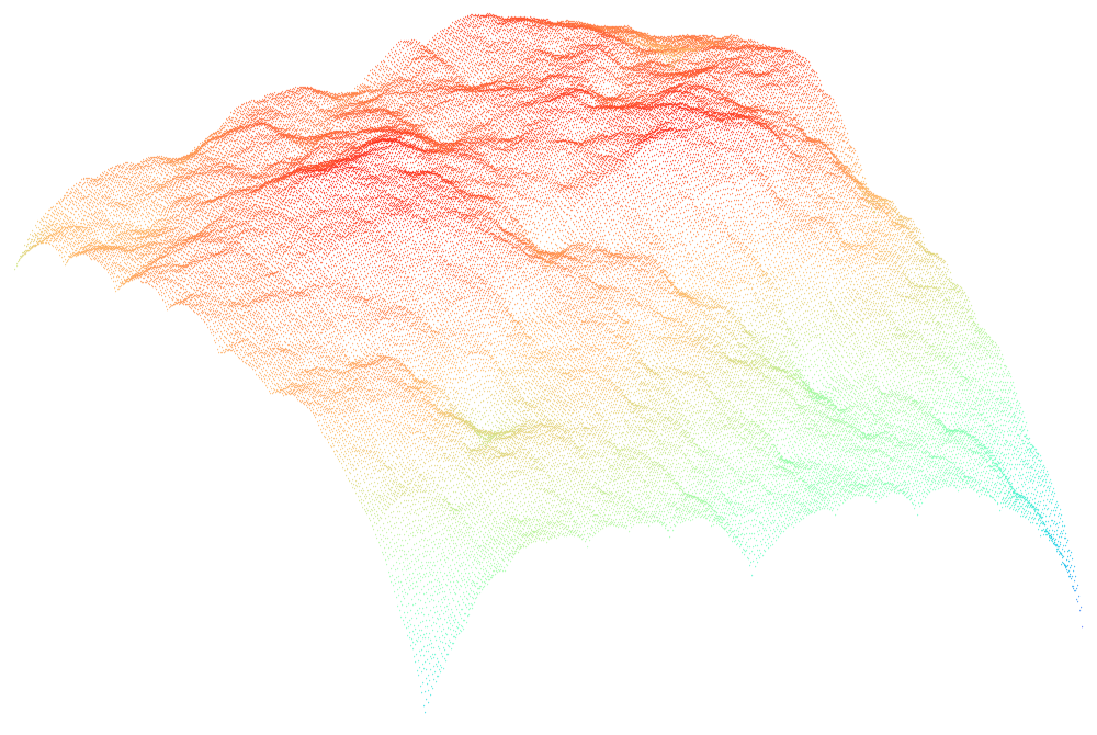
A bit faster and more efficient recursive solution generates a similar landscape:

Fig. 2. Plasma-like landscape.